"The Volatility Smile" - Derman and Miller

Amazon link

When I worked at Nortel  I occasionally got stock options.  Suppose Nortel shares were trading at $100 per share. I would be given the option of buying, say, 50 shares in six months time at a strike price of $80 per share.

Suppose Nortel stock went up in those six months to $120 per share. Those 50 shares would sell at $6,000. But I could buy them at $80, costing me $4,000.

By buying at a discount and then immediately selling, I would realise a profit of $2,000. I guess they thought I would thereby be totally incentivized to work tirelessly for stock appreciation.

As the Internet boom faded, I was seldom in the money. Nortel’s shares were under water, and my options were worthless. So at the time of issue, how should they have been priced?

Plainly the closer the option expiry date to the option trade date, the less the share price uncertainty - which lowers the option price (often called the premium).  However, if the shares are more volatile there is more chance that they will soar above the strike price - that’s got to raise the option price.

The Black-Scholes equation is a partial differential equation which describes the rate of change of option price over time as a function of stock price. The stock price is assumed to be varying as a random walk around its trend with some volatility. The equation can be solved to give option prices, similar to the call option example I discussed above.

Black-Scholes has just one unobservable parameter, the stock volatility. Other parameters in the model, the time to maturity, the strike price, the risk-free interest rate, and the current underlying stock price are all observable. In principle an option's theoretical value is a monotonically increasing function of implicit volatility.

The Black-Scholes model implies that the stock price volatility is flat compared with the strike price. This is not empirically true. When running Black-Scholes in reverse, computing the implicit volatility from observed market rates for options (and using the other observable parameters), equities tend to have skewed curves: compared to at-the-money, implied volatility is substantially higher for low strikes, and slightly lower for high strikes. Commodities often have the reverse behaviour to equities, with higher implied volatility for higher strikes. This departure from linearity, when graphed, is termed the volatility smile.

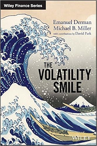
Naturally it is possible – at the expense of additional complexity – to factor in these non-linearities. And so we come to Derman’s and Miller’s book, “The Volatility Smile”. Aimed at practitioners who have already absorbed the standard Black-Scholes approach, this treatment looks in detail at several advanced models (local volatility, stochastic diffusion, jump-diffusion) which aim to provide a better match to real-life behaviour.

Presenting itself as a mathematical textbook, albeit informed and motivated by market realities, the precondition for getting the best from this work is plainly a postgraduate qualification in mathematical finance. The book is really for working quants. Those with the right background will, however, find the presentation both relevant and lucid.